numpy模块、pandas模块.基本操作、股票案例

时间：2020-07-13 23:15:42 收藏：0 阅读：72

数据分析三剑客

numpy
pandas(重点)
matplotlib

重点：

numpy数组的创建
numpy索引和切片
级联
变形
矩阵的乘法和转置
常见的聚合函数+统计

numpy的创建

使用np.array()创建
使用plt创建
使用np的routines函数创建

使用array()创建一个一维数组

import numpy as np
np.array([1,2,3,4,5])

使用array()创建一个多维数组

np.array([[1,2,3],[4,5,6]])

数组和列表的区别是什么？

数组中存储的数据元素类型必须是统一类型
优先级：
- 字符串 > 浮点型 > 整数

IN     np.array([[1,2,3],[4.4,5,6]])
OUT    array([[1. , 2. , 3. ],
             [4.4, 5. , 6. ]])  --------------------------------->浮点型


IN     np.array([[1,‘two‘,3],[4.4,5,6]])

out    array([[‘1‘, ‘two‘, ‘3‘],
             [‘4.4‘, ‘5‘, ‘6‘]], dtype=‘<U21‘)------------------->字符型

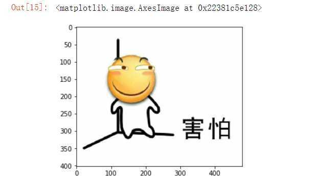
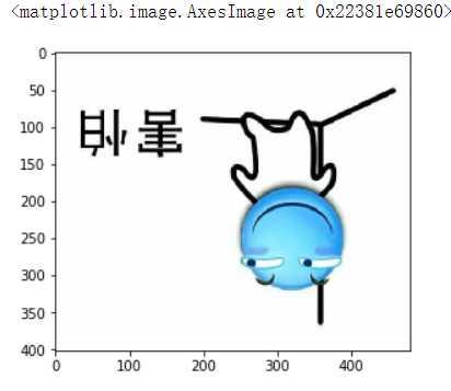
将外部的一张图片读取加载到numpy数组中，然后尝试改变数组元素的数值查看对原始图片的影响

import matplotlib.pyplot as plt
#imread可以返回一个numpy数组
img_arr = plt.imread(‘./滑稽.jpg‘)

#将返回的数组的数据进行图像的展示
plt.imshow(img_arr)

技术分享图片

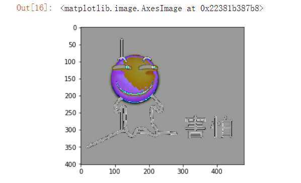
plt.imshow(img_arr - 100) 图片转换的np数组中的每个元素都-100

技术分享图片

zero()
ones()
linespace()
arange()
random系列

np.ones(shape=(3,4))         shape 形状    创建一个三行，四列的数组       zero（） 和ones() 用法一样

array([[1., 1., 1., 1.],
       [1., 1., 1., 1.],
       [1., 1., 1., 1.]])



np.linspace(0,50,num=10) #返回一维形式的等差数列   0 50 范围  num 返回元素个数

array([ 0.        ,  5.55555556, 11.11111111, 16.66666667, 22.22222222,
       27.77777778, 33.33333333, 38.88888889, 44.44444444, 50.        ])


np.arange(0,50,5)#返回一维形式的等差数列          0  20  范围  5 步数（差值）

array([ 0,  5, 10, 15, 20, 25, 30, 35, 40, 45])


np.random.randint(0,100,size=(4,5)) #返回指定形状的随机数组

array([[81, 58, 88, 25, 90],
       [65, 55,  7, 32, 36],
       [43, 30, 31, 65, 99],
       [60, 75, 58, 55, 74]])


np.random.random(size=(3,4)) #随机范围0-1

array([[0.53176578, 0.83797906, 0.49831631, 0.55847319],
       [0.33912668, 0.96287254, 0.31739383, 0.82212283],
       [0.21335858, 0.54605667, 0.69169515, 0.3366398 ]])

numpy的常用属性

shape
ndim
size
dtype

img_arr.shape #返回数组形状

(402, 480, 3)

img_arr.ndim #维度

3
img_arr.size #返回数组元素总个数

img_arr.dtype #数组元素的数据类型

dtype(‘uint8‘)

type(img_arr) #数组的类型

numpy.ndarray

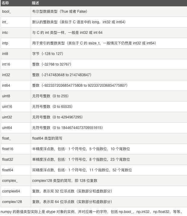
numpy的数据类型

array(dtype=?):可以设定数据类型
arr.dtype = ‘?‘:可以修改数据类型

技术分享图片

arr = np.array([1,2,3],dtype=‘float32‘)
arr

array([1., 2., 3.], dtype=float32)

#修改arr元素的数据类型
arr.astype(‘int8‘)

array([1, 2, 3], dtype=int8)

numpy的索引和切片操作（重点）

索引操作和列表同理

arr = np.random.randint(0,100,size=(5,6))
arr

array([[14, 89, 71, 96,  1, 94],
       [30, 98, 10, 64, 71, 54],
       [ 4, 80,  6, 27, 88,  3],
       [83, 75, 99, 24, 57, 37],
       [98, 24, 57, 42, 20, 21]])

arr[1][3]

切片操作

切出前两列数据
切出前两行数据
切出前两行的前两列的数据
数组数据翻转
练习：将一张图片上下左右进行翻转操作
练习：将图片进行指定区域的裁剪

#切出数组的前两行的数据
arr[0:2]

array([[14, 89, 71, 96,  1, 94],
       [30, 98, 10, 64, 71, 54]])

#切出数组的前两列
arr[:,0:2] #逗号前为行，逗号后为列

array([[14, 89],
       [30, 98],
       [ 4, 80],
       [83, 75],
       [98, 24]])

#切出前两行的前两列
arr[0:2,0:2]

array([[14, 89],
       [30, 98]])

#将数组进行倒置
arr[::-1]

array([[98, 24, 57, 42, 20, 21],
       [83, 75, 99, 24, 57, 37],
       [ 4, 80,  6, 27, 88,  3],
       [30, 98, 10, 64, 71, 54],
       [14, 89, 71, 96,  1, 94]])

#将数组进列倒置
arr[:,::-1]

array([[94,  1, 96, 71, 89, 14],
       [54, 71, 64, 10, 98, 30],
       [ 3, 88, 27,  6, 80,  4],
       [37, 57, 24, 99, 75, 83],
       [21, 20, 42, 57, 24, 98]])
#将数组进行和列都倒置
arr[::-1,::-1]

array([[21, 20, 42, 57, 24, 98],
       [37, 57, 24, 99, 75, 83],
       [ 3, 88, 27,  6, 80,  4],
       [54, 71, 64, 10, 98, 30],
       [94,  1, 96, 71, 89, 14]])

img_arr.shape

(402, 480, 3)              #402  480 是像素 也是就行和列       3控制的是颜色

#将图片进行左右翻转
plt.imshow(img_arr[:,::-1,:])

技术分享图片

plt.imshow(img_arr[::-1]) #上下倒置

技术分享图片

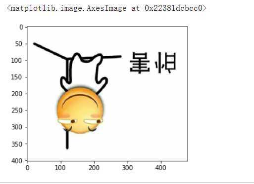
plt.imshow(img_arr[::-1,::-1,::-1]) #上下左右颜色都倒置

技术分享图片

#图片的裁剪：将脸部数据裁剪下来
plt.imshow(img_arr[80:220,90:230,:])

技术分享图片

变形reshape

注意：变形前和变形后数组的容量不可以发生变化

arr
array([[97, 52,  0, 10, 49, 90],
       [43, 96,  1, 51, 17, 12],
       [22,  9, 26, 78, 24, 59],
       [86, 85, 69, 17, 95, 37],
       [61, 61, 79, 19, 82, 98]])


arr.shape

(5, 6)

#将二维数组变形成一维数组
arr_1 = arr.reshape((30,)) #arr 是五行六列 30个元素变形前和变形后数组的容量不可以发生变化

array([97, 52,  0, 10, 49, 90, 43, 96,  1, 51, 17, 12, 22,  9, 26, 78, 24,
       59, 86, 85, 69, 17, 95, 37, 61, 61, 79, 19, 82, 98])

#将一维变多维

arr_1.reshape((6,5))

array([[14, 89, 71, 96,  1],
       [94, 30, 98, 10, 64],
       [71, 54,  4, 80,  6],
       [27, 88,  3, 83, 75],
       [99, 24, 57, 37, 98],
       [24, 57, 42, 20, 21]])

arr_1.reshape((-1,5)) #-1 表示自动匹配

array([[14, 89, 71, 96,  1],
       [94, 30, 98, 10, 64],
       [71, 54,  4, 80,  6],
       [27, 88,  3, 83, 75],
       [99, 24, 57, 37, 98],
       [24, 57, 42, 20, 21]])

级联操作

- 将多个numpy数组进行横向或者纵向的拼接

axis轴向的理解
- 0:列
- 1:行
问题：
- 级联的两个数组维度一样，但是行列个数不一样会如何？

#axis=0列和列进行拼接，axis=1行跟行进行拼接

np.concatenate((arr,arr),axis=0)   #arr 列拼接

array([[97, 52,  0, 10, 49, 90],
       [43, 96,  1, 51, 17, 12],
       [22,  9, 26, 78, 24, 59],
       [86, 85, 69, 17, 95, 37],
       [61, 61, 79, 19, 82, 98],
       [97, 52,  0, 10, 49, 90],
       [43, 96,  1, 51, 17, 12],
       [22,  9, 26, 78, 24, 59],
       [86, 85, 69, 17, 95, 37],
       [61, 61, 79, 19, 82, 98]])

 np.concatenate((arr,arr),axis=1) #arr 行拼接

array([[14, 89, 71, 96,  1, 94, 14, 89, 71, 96,  1, 94],
       [30, 98, 10, 64, 71, 54, 30, 98, 10, 64, 71, 54],
       [ 4, 80,  6, 27, 88,  3,  4, 80,  6, 27, 88,  3],
       [83, 75, 99, 24, 57, 37, 83, 75, 99, 24, 57, 37],
       [98, 24, 57, 42, 20, 21, 98, 24, 57, 42, 20, 21]])

arr_new = np.random.randint(0,100,size=(5,5))
arr_new

array([[87, 58,  2, 60, 80],
       [45, 90,  7, 83, 67],
       [90, 99, 84, 21, 49],
       [29, 92, 58, 41, 98],
       [75, 97, 64, 13, 83]])

#如果横向级联保证行数一致，纵向级联保证列数一致
#注意：维度不一致的数组无法级联
np.concatenate((arr,arr_new),axis=1)

array([[14, 89, 71, 96,  1, 94, 87, 58,  2, 60, 80],
       [30, 98, 10, 64, 71, 54, 45, 90,  7, 83, 67],
       [ 4, 80,  6, 27, 88,  3, 90, 99, 84, 21, 49],
       [83, 75, 99, 24, 57, 37, 29, 92, 58, 41, 98],
       [98, 24, 57, 42, 20, 21, 75, 97, 64, 13, 83]])

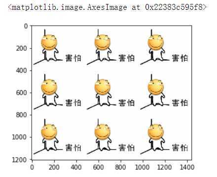
#图片的9宫格
img_arr_3 = np.concatenate((img_arr,img_arr,img_arr),axis=1) #三张图片横向拼接

技术分享图片

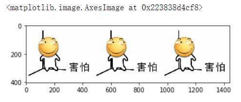
img_arr_9 = np.concatenate((img_arr_3,img_arr_3,img_arr_3),axis=0) #三张横向拼接的图再三张纵向拼接
plt.imshow(img_arr_9)

技术分享图片

常用的聚合操作

sum,max,min,mean

arr.sum()  #arr 内所有元素的和
1525
arr.sum(axis=0) #所有行的和

array([309, 303, 175, 175, 267, 296])         #sum 、 max 、 min 差不多


arr.mean(axis=0)                              #求所有行的均值

array([45.8, 73.2, 48.6, 50.6, 47.4, 41.8])

array([33.4, 51.3, 66.9])

常用的数学函数

NumPy 提供了标准的三角函数：sin()、cos()、tan()
numpy.around(a,decimals) 函数返回指定数字的四舍五入值。
- 参数说明：
  - a: 数组
  - decimals: 舍入的小数位数。默认值为0。如果为负，整数将四舍五入到小数点左侧的位置

np.sin([3,5,4,6,2,1])    # 数转正弦函数

array([ 0.14112001, -0.95892427, -0.7568025 , -0.2794155 ,  0.90929743,
        0.84147098])

np.around([33.4,51.2,66.8],decimals=-1)  #四舍五入  decimals  0  表示保留整数  -1 表示小数点外第一个数做四舍五入 即33.4的个位数3  51.6的1 做四舍五入  1 表示的是小数点最后一位做

四舍五入

array([30., 50., 70.])
np.around([33.44,51.26,66.86],decimals=1)

常用的统计函数

numpy.amin() 和 numpy.amax()，用于计算数组中的元素沿指定轴的最小、最大值。
numpy.ptp():计算数组中元素最大值与最小值的差（最大值 - 最小值）。
numpy.median() 函数用于计算数组 a 中元素的中位数（中值）
标准差std():标准差是一组数据平均值分散程度的一种度量。
- 公式：std = sqrt(mean((x - x.mean())**2))
- 如果数组是 [1，2，3，4]，则其平均值为 2.5。因此，差的平方是 [2.25,0.25,0.25,2.25]，并且其平均值的平方根除以 4，即 sqrt(5/4) ，结果为 1.1180339887498949。
方差var()：统计中的方差（样本方差）是每个样本值与全体样本值的平均数之差的平方值的平均数，即 mean((x - x.mean())** 2)。换句话说，标准差是方差的平方根。

np.median(arr,axis=0)  #求出中位数

array([30., 80., 57., 42., 57., 37.])

#标准差
arr.std(axis=1)

array([38.74453366, 28.38867145, 35.87787929, 26.04963212, 27.66867463])

矩阵相关

NumPy 中包含了一个矩阵库 numpy.matlib，该模块中的函数返回的是一个矩阵，而不是 ndarray 对象。一个的矩阵是一个由行（row）列（column）元素排列成的矩形阵列。

numpy.matlib.identity() 函数返回给定大小的单位矩阵。单位矩阵是个方阵，从左上角到右下角的对角线（称为主对角线）上的元素均为 1，除此以外全都为 0。

转置矩阵
.T
arr.T #行变列，列变行

array([[14, 30,  4, 83, 98],
       [89, 98, 80, 75, 24],
       [71, 10,  6, 99, 57],
       [96, 64, 27, 24, 42],
       [ 1, 71, 88, 57, 20],
       [94, 54,  3, 37, 21]])

矩阵相乘

numpy.dot(a, b, out=None)
- a : ndarray 数组
- b : ndarray 数组

技术分享图片

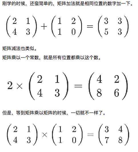
np.dot([[2,1],[4,3]],[[1,2],[1,0]])
array([[3, 4],
       [7, 8]])

pandas

为什么学习pandas

numpy已经可以帮助我们进行数据的处理了，那么学习pandas的目的是什么呢？
- numpy能够帮助我们处理的是数值型的数据，当然在数据分析中除了数值型的数据还有好多其他类型的数据（字符串，时间序列），那么pandas就可以帮我们很好的处理除了数值型的其他数据！

什么是pandas？

首先先来认识pandas中的两个常用的类
- Series
- DataFrame

Series

Series是一种类似与一维数组的对象，由下面两个部分组成：
- values：一组数据（ndarray类型）
- index：相关的数据索引标签

Series的创建
- 由列表或numpy数组创建
- 由字典创建

Series的索引

隐式索引：默认形式的索引（0，1，2....）
显示索引:自定义的索引,可以通过index参数设置显示索引

import pandas as pd
from pandas import Series,DataFrame
import numpy as np

Series(data=[1,2,3,4,5])  #data是数据源   可以是列表 也可以是字典

索引  值

0    1
1    2
2    3
3    4
4    5
dtype: int64

dic = {
‘A‘:100,
‘B‘:99,
‘C‘:120
}

Series(data=dic)

A    100
B     99
C    120
dtype: int64

Series(data=np.random.randint(0,100,size=(3,)),index=[‘A‘,‘B‘,‘C‘])

A    53
B    23
C    97
dtype: int64

Series的索引和切片

s = Series(data=np.linspace(0,30,num=5),index=[‘a‘,‘b‘,‘c‘,‘d‘,‘e‘])
s

a     0.0
b     7.5
c    15.0
d    22.5
e    30.0
dtype: float64

s[1] #通过索引
s[‘c‘] #通过显示索引显示索引也可以用点的方式点出来
s.c
s[0:3] #切片
s[‘a‘:‘d‘] #通过索引切片

a     0.0
b     7.5
c    15.0
d    22.5
dtype: float64

Series的常用属性

shape 形状
size 大小
index 索引（有显示索引是显示没有就隐式索引）
values 值

s.index
s.values

array([ 0. ,  7.5, 15. , 22.5, 30. ])

- Series的常用方法
- head(),tail()
- unique()
- isnull(),notnull()
- add() sub() mul() div()

#显示Series的前n个或者后n个元素
s.head(3) # 只显示前三个   默认是5
s.tail(2) #  只显示后两个

d    22.5
e    30.0
dtype: float64

s = Series(data=[1,1,2,2,3,3,3,3,3,3,4,5,6,7,7,7])
s.unique() #去除重复元素

array([1, 2, 3, 4, 5, 6, 7])


s.nunique() #统计去重后的元素个数

Series的算术运算

法则：索引一致的元素进行算数运算否则补空

s1 = Series(data=[1,2,3,4,5],index=[‘a‘,‘b‘,‘c‘,‘d‘,‘e‘])
s2 = Series(data=[1,2,3,4,5],index=[‘a‘,‘b‘,‘f‘,‘d‘,‘e‘])
s = s1 + s2
s                                                                索引不一样的无法+ 补空  显示NaN

a     2.0
b     4.0
c     NaN
d     8.0
e    10.0
f     NaN
dtype: float64

s.isnull() #检测Series哪些元素为空，为空则返回True，否则返回False

a    False
b    False
c     True
d    False
e    False
f     True
dtype: bool


s.notnull() #哪些元素为非空，返回True，否则返回False

a     True
b     True
c    False
d     True
e     True
f    False
dtype: bool

a     2.0
b     4.0
c     NaN
d     8.0
e    10.0
f     NaN
dtype: float64

#想要将s中的非空的数据取出
s[[True,True,False,True,True,False]]

a     2.0
b     4.0
d     8.0
e    10.0
dtype: float64


s[s.notnull()] #可以对Series中的空值进行清洗

a     2.0
b     4.0
d     8.0
e    10.0
dtype: float64

DataFrame

DataFrame是一个【表格型】的数据结构。DataFrame由按一定顺序排列的多列数据组成。设计初衷是将Series的使用场景从一维拓展到多维。DataFrame既有行索引，也有列索引。
- 行索引：index
- 列索引：columns
- 值：values

DataFrame的创建
- ndarray创建
- 字典创建

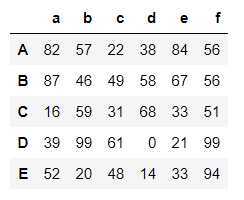
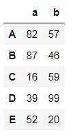
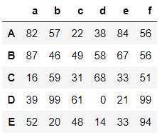
df = DataFrame(data=np.random.randint(0,100,size=(5,6)),columns=[‘a‘,‘b‘,‘c‘,‘d‘,‘e‘,‘f‘],index=[‘A‘,‘B‘,‘C‘,‘D‘,‘E‘])

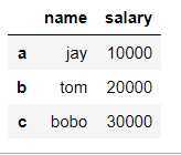
dic = {
‘name‘:[‘jay‘,‘tom‘,‘bobo‘],
‘salary‘:[10000,20000,30000]
}
DataFrame(data=dic,index=[‘a‘,‘b‘,‘c‘])

技术分享图片

DataFrame的属性

values、columns、index、shape

df.values #返回元素
df.columns #列索引
df.index   #行索引
df.shape   #形状

DataFrame索引操作

对行进行索引
队列进行索引
对元素进行索引

df

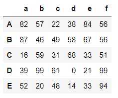
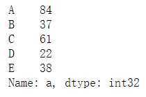
#对列进行索引(只可以使用显示列索引)
df[‘a‘]

技术分享图片

df[[‘a‘,‘b‘]] #取多列

技术分享图片

iloc:
- 通过隐式索引取行
loc:
- 通过显示索引取行

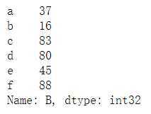
#索引取行
df.loc[‘B‘]   #显示索引
df.iloc[1]    #隐式索引

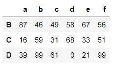
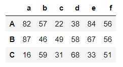
#取出多行
df.iloc[[1,2,3]]

#取出元素
df.loc[‘B‘,‘e‘]

#取多个元素
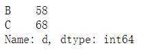
df.iloc[[1,2],3] # 取出 2 3 两行第三列的元素

技术分享图片

DataFrame的切片操作

对行进行切片
对列进行切片

df

#切行
df[0:3]

#切列
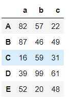
df.iloc[:,0:3]

技术分享图片

df索引和切片操作
- 索引：
  - df[col]:取列
  - df.loc[index]:取行
  - df.iloc[index,col]:取元素
- 切片：
  - df[index1:index3]:切行
  - df.iloc[:,col1:col3]:切列

DataFrame的运算
- 同Series

============================================

练习4：

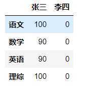
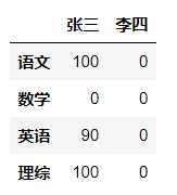
根据以下考试成绩表，创建一个DataFrame，命名为df：

    张三  李四  
语文 100  0
数学 90  0
英语 90  0
理综 100  0

假设ddd是期中考试成绩，ddd2是期末考试成绩，请自由创建ddd2，并将其与ddd相加，求期中期末平均值。
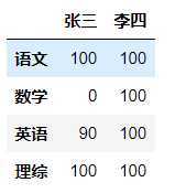
假设张三期中考试数学被发现作弊，要记为0分，如何实现？
李四因为举报张三作弊立功，期中考试所有科目加100分，如何实现？
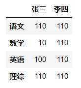
后来老师发现有一道题出错了，为了安抚学生情绪，给每位学生每个科目都加10分，如何实现？

============================================

dic = {
    ‘张三‘:[100,90,90,100],
    ‘李四‘:[0,0,0,0]
}
df = DataFrame(data=dic,index=[‘语文‘,‘数学‘,‘英语‘,‘理综‘])
qizhong = df
qimo = df

(qizhong + qimo) / 2 #平均成绩

#假设张三期中考试数学被发现作弊，要记为0分，如何实现
qizhong.loc[‘数学‘,‘张三‘] = 0
qizhong

技术分享图片

#李四因为举报张三作弊立功，期中考试所有科目加100分，如何实现
qizhong[‘李四‘] += 100
qizhong

技术分享图片

#给每位学生每个科目都加10分
qizhong += 10
qizhong

技术分享图片

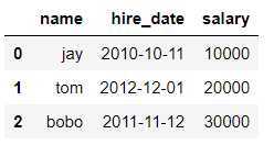
时间数据类型的转换
- pd.to_datetime(col)
将某一列设置为行索引
- df.set_index()

dic = {
    ‘name‘:[‘jay‘,‘tom‘,‘bobo‘],
    ‘hire_date‘:[‘2010-10-11‘,‘2012-12-01‘,‘2011-11-12‘],
    ‘salary‘:[10000,20000,30000]
}
df = DataFrame(data=dic)
df

#info返回df的基本信息
df.info()

<class ‘pandas.core.frame.DataFrame‘>
RangeIndex: 3 entries, 0 to 2
Data columns (total 3 columns):
name         3 non-null object       #在数据分析中  字符串 可以是 object 也可是 str
hire_date    3 non-null object
salary       3 non-null int64
dtypes: int64(1), object(2)
memory usage: 152.0+ bytes

#想要将字符串形式的时间数据转换成时间序列类型
df[‘hire_date‘] = pd.to_datetime(df[‘hire_date‘])

df.info()

<class ‘pandas.core.frame.DataFrame‘>
RangeIndex: 3 entries, 0 to 2
Data columns (total 3 columns):
name         3 non-null object
hire_date    3 non-null datetime64[ns]     ------------------------------------------------->字符串类型变成了时间序列类型
salary       3 non-null int64
dtypes: datetime64[ns](1), int64(1), object(1)
memory usage: 152.0+ bytes

#想要将hire_date列作为源数据的行索引
new_df = df.set_index(‘hire_date‘)
new_df

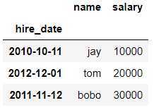
new_df.shape

(3, 2)           ------------------------>由于 原来的hire_date 变成了索引 现在 就只要三行两列了

DataFrame基础操作巩固-股票分析

tushare财经数据接口包

pip install tushare
作用：提供相关指定的财经数据

需求：股票分析

使用tushare包获取某股票的历史行情数据。
输出该股票所有收盘比开盘上涨3%以上的日期。
输出该股票所有开盘比前日收盘跌幅超过2%的日期。
假如我从2010年1月1日开始，每月第一个交易日买入1手股票，每年最后一个交易日卖出所有股票，到今天为止，我的收益如何？

import tushare as ts
import pandas as pd
from pandas import Series,DataFrame
import numpy as np

#使用tushare包获取某股票的历史行情数据。
df = ts.get_k_data(code=‘600519‘,start=‘1999-01-10‘)
df

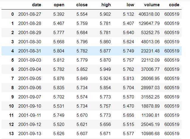技术分享图片（太多了只截一部分）

df的持久化存储

df.to_xxx()

#将df的数据存储到本地
df.to_csv(‘./maotai.csv‘)

#加载外部数据到df中：read_xxx()
df = pd.read_csv(‘./maotai.csv‘)
df.head()

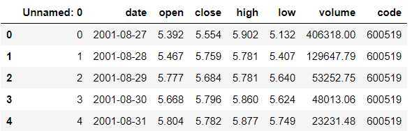
#将Unnamed: 0列进行删除
#在drop系列的函数中axis=0表示的行，1表示的是列
df.drop(labels=‘Unnamed: 0‘,axis=1,inplace=True)

#查看数据的原始信息
df.info()

<class ‘pandas.core.frame.DataFrame‘>
RangeIndex: 4503 entries, 0 to 4502
Data columns (total 7 columns):
date      4503 non-null object
open      4503 non-null float64
close     4503 non-null float64
high      4503 non-null float64
low       4503 non-null float64
volume    4503 non-null float64
code      4503 non-null int64
dtypes: float64(5), int64(1), object(1)
memory usage: 246.3+ KB

#将date列的字符串类型的时间转换成时间序列类型
df[‘date‘] = pd.to_datetime(df[‘date‘])

df[‘date‘].dtype

dtype(‘<M8[ns]‘)

#将date列作为源数据的行索引
df.set_index(keys=‘date‘,inplace=True)

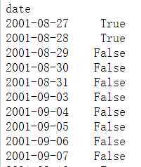
#输出该股票所有收盘比开盘上涨3%以上的日期。
#(收盘-开盘)/开盘 > 0.03
(df[‘close‘] - df[‘open‘]) / df[‘open‘] > 0.03

技术分享图片 ]

#经验：在df的相关操作中如果一旦返回了布尔值，下一步马上将布尔值作为原始数据的行索引

#发现布尔值可以作为df的行索引，可以直接取出true对应的行数据
df.loc[[True,True,False,False,True]]

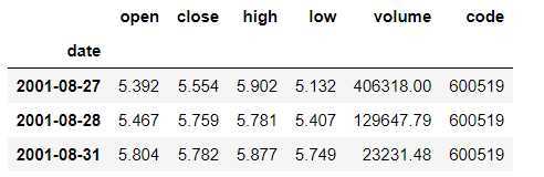
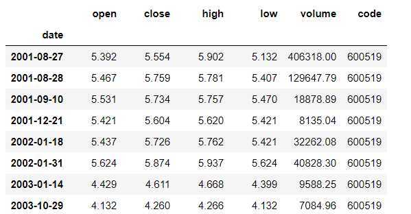
#将满足需求的行数据获取（收盘比开盘上涨3%以上）
df.loc[(df[‘close‘] - df[‘open‘]) / df[‘open‘] > 0.03]

#获取满足要求的日期
df.loc[(df[‘close‘] - df[‘open‘]) / df[‘open‘] > 0.03].index

DatetimeIndex([‘2001-08-27‘, ‘2001-08-28‘, ‘2001-09-10‘, ‘2001-12-21‘,
               ‘2002-01-18‘, ‘2002-01-31‘, ‘2003-01-14‘, ‘2003-10-29‘,
               ‘2004-01-05‘, ‘2004-01-14‘,
               ...
               ‘2020-03-02‘, ‘2020-03-05‘, ‘2020-03-10‘, ‘2020-04-02‘,
               ‘2020-04-22‘, ‘2020-05-06‘, ‘2020-05-18‘, ‘2020-07-02‘,
               ‘2020-07-06‘, ‘2020-07-07‘],
              dtype=‘datetime64[ns]‘, name=‘date‘, length=314, freq=None)

#输出该股票所有开盘比前日收盘跌幅超过2%的日期。
#(开盘 - 前日收盘) / 前日收盘 < -0.02
(df[‘open‘] - df[‘close‘].shift(1)) / df[‘close‘].shift(1) < -0.02
df.loc[(df[‘open‘] - df[‘close‘].shift(1)) / df[‘close‘].shift(1) < -0.02]
df.loc[(df[‘open‘] - df[‘close‘].shift(1)) / df[‘close‘].shift(1) < -0.02].index

假如我从2010年1月1日开始，每月第一个交易日买入1手(100支)股票，每年最后一个交易日卖出所有股票，到今天为止，我的收益如何？

买股票
- 每月的第一个交易日根据开盘价买入一手股票
- 一个完整的年需要买入12次12手1200支股票
卖股票
- 每年最后一个交易日根据开盘价(12-31)卖出所有的股票
- 一个完整的年需要卖出1200支股票
注意：2020年这个人只能买入700支股票，无法卖出。但是在计算总收益的时候需要将剩余股票的价值也计算在内
- 剩余股票价值如何计算：
  - 700 * 买入当日的开盘价

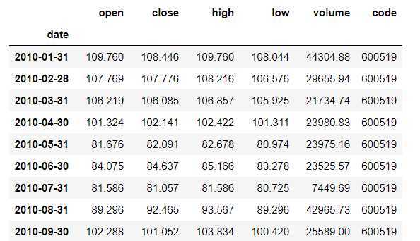
new_df = df[‘2010‘:‘2020‘] #如果行索引为时间序列类型数据

#数据的重新取样resample
df_monthly = new_df.resample(rule=‘M‘).first()
df_monthly#每一个月第一个交易日对应的行数据

#计算买入股票一共花了多少钱
cost = df_monthly[‘open‘].sum() * 100
cost

4636917.100000001

#求出卖出股票收入多少钱:A表示的是年
df_yearly = new_df.resample(‘A‘).last()[0:-1]
df_yearly#存储的是每一年最后一个交易日对应的行数据

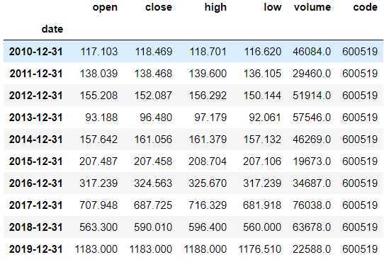
recv = df_yearly[‘open‘].sum() * 1200
recv

4368184.8

#求出剩余股票的价值
last = 700 * df[‘open‘][-1]

#总收益
recv + last - cost

913567.6999999993

需求：双均线策略制定

使用tushare包获取某股票的历史行情数据

计算该股票历史数据的5日均线和30日均线

什么是均线？
- 对于每一个交易日，都可以计算出前N天的移动平均值，然后把这些移动平均值连起来，成为一条线，就叫做N日移动平均线。移动平均线常用线有5天、10天、30天、60天、120天和240天的指标。
  - 5天和10天的是短线操作的参照指标，称做日均线指标；
  - 30天和60天的是中期均线指标，称做季均线指标；
  - 120天和240天的是长期均线指标，称做年均线指标。
均线计算方法：MA=（C1+C2+C3+...+Cn)/N C:某日收盘价 N:移动平均周期（天数）


分析输出所有金叉日期和死叉日期

股票分析技术中的金叉和死叉，可以简单解释为：
- 分析指标中的两根线，一根为短时间内的指标线，另一根为较长时间的指标线。
- 如果短时间的指标线方向拐头向上，并且穿过了较长时间的指标线，这种状态叫“金叉”；
- 如果短时间的指标线方向拐头向下，并且穿过了较长时间的指标线，这种状态叫“死叉”；
- 一般情况下，出现金叉后，操作趋向买入；死叉则趋向卖出。当然，金叉和死叉只是分析指标之一，要和其他很多指标配合使用，才能增加操作的准确性。

如果我从假如我从2010年1月1日开始，初始资金为100000元，金叉尽量买入，死叉全部卖出，则到今天为止，我的炒股收益率如何？
分析：
- 买卖股票的单价使用开盘价
- 买卖股票的时机
- 最终手里会有剩余的股票没有卖出去
  - 会有。如果最后一天为金叉，则买入股票。估量剩余股票的价值计算到总收益。
    - 剩余股票的单价就是用最后一天的收盘价。

原文：https://www.cnblogs.com/linranran/p/13296374.html